Equations of motion for a particle

Equations of motion for a particle

We start with some basic definitions and physical laws.

1 Definition of a particle

A `Particle’ is a point mass at some position in space. It can move about, but has no characteristic orientation or rotational inertia.  It is characterized by its mass.

Examples of applications where you might choose to idealize part of a system as a particle include:

1.      Calculating the orbit of a satellite  for this application, you don’t need to know the orientation of the satellite, and you know that the satellite is very small compared with the dimensions of its orbit.

2.      A molecular dynamic simulation, where you wish to calculate the motion of individual atoms in a material.  Most of the mass of an atom is usually concentrated in a very small region (the nucleus) in comparison to inter-atomic spacing. It has negligible rotational inertia.   This approach is also sometimes used to model entire molecules, but rotational inertia can be important in this case.

Obviously, if you choose to idealize an object as a particle, you will only be able to calculate its position.  Its orientation or rotation cannot be computed.

2 Position, velocity, acceleration relations for a particle (Cartesian coordinates)

In most practical applications we are interested in the position or the velocity (or speed) of the particle as a function of time.   But Newton’s laws will only tell us its acceleration.   We therefore need equations that relate the position, velocity and acceleration.

Position vector: In most of the problems we solve in this course, we will specify the position of a particle using the Cartesian components of its position vector with respect to a convenient origin.  This means

1.      We choose three, mutually perpendicular, fixed directions in space.  The three directions are described by unit vectors 

2.      We choose a convenient point to use as origin.

3.      The position vector (relative to the origin) is then specified by the three distances (x,y,z) shown in the figure.

In dynamics problems, all three components can be functions of time.

Velocity vector: By definition, the velocity is the derivative of the position vector with respect to time (following the usual machinery of calculus)

Velocity is a vector, and can therefore be expressed in terms of its Cartesian components

You can visualize a velocity vector as follows

·         The direction of the vector is parallel to the direction of motion

·         The magnitude of the vector  is the speed of the particle (in meters/sec, for example). 

When both position and velocity vectors are expressed in terms Cartesian components, it is simple to calculate the velocity from the position vector.   For this case, the basis vectors  are constant (independent of time) and so

This is really three equations  one for each velocity component, i.e.

Acceleration vector: The acceleration is the derivative of the velocity vector with respect to time; or, equivalently, the second derivative of the position vector with respect to time.

The acceleration is a vector, with Cartesian representation .

Like velocity, acceleration has magnitude and direction. Sometimes it may be possible to visualize an acceleration vector  for example, if you know your particle is moving in a straight line, the acceleration vector must be parallel to the direction of motion; or if the particle moves around a circle at constant speed, its acceleration is towards the center of the circle.  But sometimes you can’t trust your intuition regarding the magnitude and direction of acceleration, and it can be best to simply work through the math.

The relations between Cartesian components of position, velocity and acceleration are

3 Examples using position-velocity-acceleration relations

It is important for you to be comfortable with calculating velocity and acceleration from the position vector of a particle.   You will need to do this in nearly every problem we solve.  In this section we provide a few examples.  Each example gives a set of formulas that will be useful in practical applications.

Example 1: Constant acceleration along a straight line.  There are many examples where an object moves along a straight line, with constant acceleration.   Examples include free fall near the surface of a planet (without air resistance), the initial stages of the acceleration of a car, or and aircraft during takeoff roll, or a spacecraft during blastoff.

Suppose that

The particle moves parallel to a unit vector i

The particle has constant acceleration, with magnitude a

At time  the particle has speed 

At time  the particle has position vector 

The position, velocity acceleration vectors are then

Verify for yourself that the position, velocity and acceleration (i) have the correct values at t=0 and (ii) are related by the correct expressions (i.e. differentiate the position and show that you get the correct expression for the velocity, and differentiate the velocity to show that you get the correct expression for the acceleration).

HEALTH WARNING: These results can only be used if the acceleration is constant.  In many problems acceleration is a function of time, or position  in this case these formulas cannot be used. People who have taken high school physics classes have used these formulas to solve so many problems that they automatically apply them to everything  this works for high school problems but not always in real life!

Example 2: Simple Harmonic Motion:  The vibration of a very simple spring-mass system is an example of simple harmonic motion.

In simple harmonic motion (i) the particle moves along a straight line; and (ii) the position, velocity and acceleration are all trigonometric functions of time.

For example, the position vector of the mass might be given by

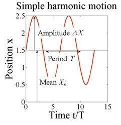
Here  is the average length of the spring,  is the maximum length of the spring, and T is the time for the mass to complete one complete cycle of oscillation (this is called the `period’ of oscillation). 

Harmonic vibrations are also often characterized by the frequency of vibration:

·         The frequency in cycles per second (or Hertz) is related to the period by f=1/T

·         The angular frequency is related to the period by 

The motion is plotted in the figure on the right.

The velocity and acceleration can be calculated by differentiating the position, as follows

Note that:

·         The velocity and acceleration are also harmonic, and have the same period and frequency as the displacement.

·         If you know the frequency, and amplitude and of either the displacement, velocity, or acceleration, you can immediately calculate the amplitudes of the other two.  For example, if , ,  denote the amplitudes of the displacement, velocity and acceleration, we have that

Example 3: Motion at constant speed around a circular path  Circular motion is also very common  examples include any rotating machinery, vehicles traveling around a circular path, and so on.

The simplest way to make an object move at constant speed along a circular path is to attach it to the end of a shaft (see the figure), and then rotate the shaft at a constant angular rate.  Then, notice that

·       The angle  increases at constant rate.  We can write , where  is the (constant) angular speed of the shaft, in radians/seconds. 

·       The speed of the particle is related to  by .   To see this, notice that the circumferential distance traveled by the particle is .  Therefore, .

For this example the position vector is

The velocity can be calculated by differentiating the position vector. 

Here, we have used the chain rule of differentiation, and noted that .

The acceleration vector follows as

Note that

 (i) The magnitude of the velocity is , and its direction is (obviously!) tangent to the path (to see this, visualize (using trig) the direction of the unit vector 

(ii) The magnitude of the acceleration is  and its direction is towards the center of the circle. To see this, visualize (using trig) the direction of the unit vector  

We can write these mathematically as

Example 4: More general motion around a circular path 

We next look at more general circular motion, where the particle still moves around a circular path, but does not move at constant speed.  The angle  is now a general function of time. 

We can write down some useful scalar relations:

·       Angular rate: 

·       Angular acceleration 

·       Speed 

·       Rate of change of speed 

We can now calculate vector velocities and accelerations

The velocity can be calculated by differentiating the position vector. 

The acceleration vector follows as

It is often more convenient to re-write these in terms of the unit vectors n and t normal and tangent to the circular path, noting that , .  Then

These are the famous circular motion formulas that you might have seen in physics class. 

 4 Velocity and acceleration in normal-tangential and cylindrical polar coordinates.

In some cases it is helpful to use special basis vectors to write down velocity and acceleration vectors, instead of a fixed {i,j,k} basis.  If you see that this approach can be used to quickly solve a problem  go ahead and use it.  If not, just use Cartesian coordinates  this will always work, and with Mathematica is not very hard.  The only benefit of using the special coordinate systems is to save a couple of lines of rather tedious trigonometric algebra  which can be extremely helpful when solving an exam question, but is generally insignificant when solving a real problem.

Normal-tangential coordinates for particles moving along a prescribed planar path

                         

In some problems, you might know the particle speed, and the x,y coordinates of the path (a car traveling along a road is a good example).   In this case it is often easiest to use normal-tangentialcoordinates to describe forces and motion. 

For this purpose we

·       Introduce two unit vectors n and t, with t pointing tangent to the path and n pointing normal to the path, towards the center of curvature

·       Introduce the radius of curvature of the path R.

Then:

(i)                 The direction of the velocity vector of a particle is tangent to its path.  The magnitude of the velocity vector is equal to the speed.

(ii)               The acceleration vector can be constructed by adding two components:

·         the component of acceleration tangent to the particle’s path is equal 

·         The component of acceleration perpendicular to the path (towards the center of curvature) is equal to .

Mathematically 

To use these formulas, you need to be able to find n, t, and R. Often you can just write these down. If you happen to know the parametric equation of the path (i.e. the x,y coordinates are known in terms of some variable  ), then

The sign of n should be selected so that

The radius of curvature can be computed from

The radius of curvature is always positive.

Example: Design speed limit for a curvy road:  As a consulting firm specializing in highway design, we have been asked to develop a design formula that can be used to calculate the speed limit for cars that travel along a curvy road.

The following procedure will be used:

·         The curvy road will be approximated as a sine wave  as shown in the figure  for a given road, engineers will measure values of Aand L that fit the path.

·         Vehicles will be assumed to travel at constant speed V around the path  your mission is to calculate the value of V

·         For safety, the magnitude of the acceleration of the car at any point along the path must be less than 0.2g, where g is the gravitational acceleration. (Again, note that constant speed does not mean constant acceleration, because the car’s direction is changing with time).

Our goal, then, is to calculate a formula for the magnitude of the acceleration in terms of V, A and L.  The result can be used to deduce a formula for the speed limit.

Calcluation:

We can solve this problem quickly using normal-tangential coordinates.  Since the speed is constant, the acceleration vector is

The position vector is , so we can calculate the radius of curvature from the formula

Note that x acts as the parameter  for this problem, and , so

and the acceleration is

We are interested in the magnitude of the acceleration… 

We see from this that the car has the biggest acceleration when . The maximum acceleration follows as

The formula for the speed limit is therefore 

Now we send in a bill for a big consulting fee…

Polar coordinates for particles moving in a plane

When solving problems involving central forces (forces that attract particles towards a fixed point) it is often convenient to describe motion using polar coordinates.

Polar coordinates are related to x,y coordinates through

Suppose that the position of a particle is specified by its ‘polar coordinates’  relative to a fixed origin, as shown in the figure. Let  be a unit vector pointing in the radial direction, and let  be a unit vector pointing in the tangential direction, i.e

The velocity and acceleration of the particle can then be expressed as

You can derive these results very easily by writing down the position vector of the particle in the {i,j} basis in terms of , differentiating, and then simplifying the results.   The details are left as an exercise.

Example The robotic manipulator shown in the figure rotates with constant angular speed  about the k axis.   Find a formula for the maximum allowable (constant) rate of extension  if the acceleration of the gripper may not exceed g.

We can simply write down the acceleration vector, using polar coordinates.  We identify  and r=L, so that

3.1.5 Measuring position, velocity and acceleration

If you are designing a control system, you will need some way to detect the motion of the system you are trying to control.  A vast array of different sensors is available for you to choose from: see for example the list athttp://www.sensorland.com/HowPage001.html .  A very short list of common sensors is given below

1.      GPS  determines position on the earth’s surface by measuring the time for electromagnetic waves to travel from satellites in known positions in space to the sensor.   Can be accurate down to cm distances, but the sensor needs to be left in position for a long time for this kind of accuracy.  A few m is more common.

2.      Optical or radio frequency position sensing  measure position by (a) monitoring deflection of laser beams off a target; or measuring the time for signals to travel from a set of radio emitters with known positions to the sensor.  Precision can vary from cm accuracy down to light wavelengths.

3.      Capacitative displacement sensing  determine position by measuring the capacitance between two parallel plates.  The device needs to be physically connected to the object you are tracking and a reference point. Can only measure distances of mm or less, but precision can be down to micron accuracy.

4.      Electromagnetic displacement sensing  measures position by detecting electromagnetic fields between conducting coils, or coil/magnet combinations within the sensor.  Needs to be physically connected to the object you are tracking and a reference point.  Measures displacements of order cm down to microns.

5.      Radar velocity sensing  measures velocity by detecting the change in frequency of electromagnetic waves reflected off the traveling object.

6.      Inertial accelerometers: measure accelerations by detecting the deflection of a spring acting on a mass.

Accelerometers are also often used to construct an ‘inertial platform,’ which uses gyroscopes to maintain a fixed orientation in space, and has three accelerometers that can detect motion in three mutually perpendicular directions.  These accelerations can then be integrated to determine the position.  They are used in aircraft, marine applications, and space vehicles where GPS cannot be used.

6 Newton’s laws of motion for a particle

Newton’s laws for a particle are very simple.  Let

1.      m denote the mass of the particle

2.      F denote the resultant force acting on the particle (as a vector)

3.      a denote the acceleration of the particle (again, as a vector).  Then

Occasionally, we use a particle idealization to model systems which, strictly speaking, are not particles.  These are:

1.      A large mass, which moves without rotation (e.g. a car moving along a straight line)

2.      A single particle which is attached to a rigid frame with negligible mass (e.g. a person on a bicycle)

In these cases it may be necessary to consider the moments acting on the mass (or frame) in order to calculate unknown reaction forces. 

1.      For a large mass which moves without rotation, the resultant moment of external forces about the center of mass must vanish.

2.      For a particle attached to a massless frame, the resultant moment of external forces acting on the frame about the particle must vanish.

It is very important to take moments about the correct point in dynamics problems! Forgetting this is the most common reason to screw up a dynamics problem…

If you need to solve a problem where more than one particle is attached to a massless frame, you have to draw a separate free body diagram for each particle, and for the frame.   The particles must obey Newton’s laws .   The forces acting on the frame must obey  and , (because the frame has no mass). 

 

 

The Newtonian Inertial Frame.

Newton’s laws are very familiar, and it is easy to write them down without much thought.  They do have a flaw, however.

When we use Newton’s laws, we assume that we can identify a convenient origin somewhere that we regard as `fixed’.   In addition, to write down an acceleration vector, we need to be able to choose a set of fixed directions in space.

For engineering calculations, this usually poses no difficulty.  If we are solving problems involving terrestrial motion over short distances compared with the earth’s radius, we simply take a point on the earth’s surface as fixed, and take three directions relative to the earth’s surface to be fixed.  If we are solving problems involving motion in space near the earth, or modeling weather, we take the center of the earth as a fixed point, (or for more complex calculations the center of the sun); and choose axes to have a fixed direction relative to nearby stars.

But in reality, an unambiguous inertial frame does not exist.  We can only describe the relative motion of the mass in the universe, not its absolute motion.  The general theory of relativity addresses this problem  and in doing so explains many small but noticeable discrepancies between the predictions of Newton’s laws and experiment.